How to Find Variance in Excel

Summary

In the example shown, column B contains delivery times in minutes for 10 orders. The formula in E5 is:

=VAR.S(B5:B14)

The result is 20.04. The formula in E6 calculates population variance instead:

=VAR.P(B5:B14)

The result is 18.04. Both formulas use the same data. The only difference is whether Excel treats the data as a sample or as the entire population.

Generic formula

=VAR.S(range)   sample variance
=VAR.P(range)   population variance

Explanation

In this example, the goal is to measure how spread out the delivery times are. Variance measures how far values are from their average. A small variance means the values sit close to the average. A large variance means the values are spread out.

The data looks like this:

Order	Minutes
1	32
2	28
3	35
4	30
5	41
6	27
7	33
8	29
9	38
10	31

The average delivery time is 32.4 minutes. Variance tells us how much the individual times move away from that average.

Which variance function should I use?

Excel has six variance functions. In most cases you only need two of them, VAR.S and VAR.P.

Function	Data treated as	Text and TRUE/FALSE in a range	Notes
VAR.S	Sample	Ignored	Use this most of the time
VAR.P	Population	Ignored	Use when you have every value
VARA	Sample	Text and FALSE = 0, TRUE = 1	Includes non-numeric values
VARPA	Population	Text and FALSE = 0, TRUE = 1	Population version of VARA
VAR	Sample	Ignored	Older function, replaced by VAR.S
VARP	Population	Ignored	Older function, replaced by VAR.P

Microsoft keeps VAR and VARP only so that older workbooks still work, and notes they may not be available in future versions of Excel. VAR.S and VAR.P are available in Excel for Microsoft 365, Excel 2024, 2021, 2019, and 2016 on Windows and Mac.

VAR.S vs VAR.P

The choice depends on what your data represents:

• Use VAR.S when your data is a sample taken from a larger group. For example, 50 customers surveyed out of thousands, or 20 days of stock returns out of many years.
• Use VAR.P when your data includes every member of the group you care about. For example, the test scores of every student in one class.

If you are not sure, use VAR.S. Real-world data is usually a sample, and Microsoft’s own guidance is to use VAR.P only when your data represents the entire population.

How to find sample variance with VAR.S

1. Enter your numbers in a single column. In the example, the values are in B5:B14.
2. Click an empty cell where you want the result.
3. Type =VAR.S(
4. Select the range B5:B14 with your mouse, or type it in.
5. Type ) and press Enter.

Excel returns 20.04.

Note: always start with an equal sign (=). Without it, Excel treats the entry as text instead of a formula.

How to find population variance with VAR.P

The steps are the same. Only the function name changes:

=VAR.P(B5:B14)

Excel returns 18.04. For the same data, the population result is smaller than the sample result (unless every value is identical), because of how each one divides the total. The next section shows why.

Variance across more than one range

VAR.S and VAR.P accept up to 255 arguments. This means you can include ranges that are not next to each other:

=VAR.S(B5:B14,D5:D14)

Arguments can be numbers, names, arrays, or cell references.

How Excel calculates variance

Excel uses these formulas:

• Sample variance (VAR.S): Σ(x – x̄)² ÷ (n – 1)
• Population variance (VAR.P): Σ(x – x̄)² ÷ n

Here, x is each value, x̄ is the average, and n is the number of values. Sample variance divides by n – 1 instead of n. This adjustment makes the sample result an unbiased estimate of the population variance.

Check the result manually

You can rebuild the calculation in a few columns to see exactly where the number comes from.

Minutes (x)	Deviation (x – 32.4)	Squared deviation
32	-0.4	0.16
28	-4.4	19.36
35	2.6	6.76
30	-2.4	5.76
41	8.6	73.96
27	-5.4	29.16
33	0.6	0.36
29	-3.4	11.56
38	5.6	31.36
31	-1.4	1.96
Total		180.40

1. Calculate the average: =AVERAGE(B5:B14) returns 32.4.
2. In C5, calculate the deviation: =B5-AVERAGE($B$5:$B$14), then copy down.
3. In D5, square the deviation: =C5^2, then copy down.
4. Add the squared deviations: =SUM(D5:D14) returns 180.40.
5. Divide by n – 1 for a sample: 180.40 ÷ 9 = 20.04. This matches VAR.S.
6. Divide by n for a population: 180.40 ÷ 10 = 18.04. This matches VAR.P.

Excel can also do steps 1 to 4 in one formula with the DEVSQ function:

=DEVSQ(B5:B14)

DEVSQ returns 180.40, the sum of squared deviations.

Variance and standard deviation

Variance is measured in squared units. In this example, the variance is 20.04 “minutes squared”, which is hard to picture. This is why many people take the next step and calculate the standard deviation, which is in the same units as the data.

Standard deviation is the square root of variance. You can calculate it in two ways:

=STDEV.S(B5:B14)
=SQRT(VAR.S(B5:B14))

Both return 4.48 minutes. For a population, use STDEV.P or =SQRT(VAR.P(B5:B14)), which return 4.25.

Reading the result

The average plus and minus one standard deviation gives a practical “normal” range:

• 32.4 – 4.48 = 27.92 minutes
• 32.4 + 4.48 = 36.88 minutes

Most deliveries fall between about 28 and 37 minutes. Orders outside this range, like the 41 minute delivery, are worth a closer look. MIN and MAX help here too: =MIN(B5:B14) returns 27 and =MAX(B5:B14) returns 41.

When to use VARA

VAR.S looks only at numbers in a range. VARA also counts text and logical values:

• Text is evaluated as 0
• TRUE is evaluated as 1
• FALSE is evaluated as 0

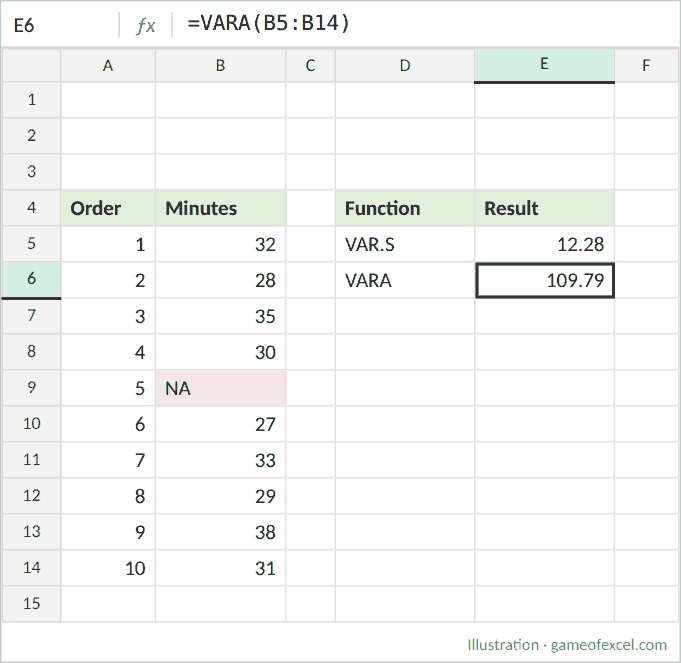
This can change the result a lot. In the example below, the value in B9 has been replaced with the text “NA”:

=VAR.S(B5:B14)   returns 12.28
=VARA(B5:B14)    returns 109.79

VAR.S ignores “NA” and uses the remaining 9 numbers. VARA treats “NA” as a zero delivery time, which pulls the variance up sharply. Use VARA only when text or TRUE/FALSE entries really should count as values. VARPA works the same way for a population.

Note: Microsoft’s documentation also says that logical values and numbers written as text are counted by VAR.S when you type them directly into the formula, for example =VAR.S(10,"12",TRUE). When they sit inside a cell range, VAR.S ignores them.

How to find variance in Excel without a formula

Analysis ToolPak

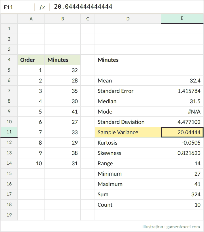
The Analysis ToolPak includes a Descriptive Statistics tool that reports variance along with other statistics.

1. Load the add-in. On Windows, go to File > Options > Add-Ins, choose Excel Add-ins in the Manage box, click Go, check Analysis ToolPak, and click OK. On Mac, go to Tools > Excel Add-ins.
2. Go to Data > Data Analysis and choose Descriptive Statistics.
3. Set the Input Range to B4:B14, check Labels in first row, and check Summary statistics.
4. Click OK.

Excel creates a table that includes the mean, standard deviation, range, minimum, maximum, and count. The variance appears in the Sample Variance row. The ToolPak always reports sample variance, which matches VAR.S.

PivotTable

A PivotTable can summarize values by variance.

1. Create a PivotTable from your data.
2. Add the value field to the Values area.
3. Right-click a value and choose Value Field Settings.
4. On the Summarize Values By tab, choose Var for a sample or Varp for a population.
5. Click OK.

This is useful when you need the variance for each category, such as each region or product.

Note: the status bar at the bottom of Excel can show the average, count, sum, minimum, and maximum, but it does not show variance.

Common problems and fixes

#DIV/0! error

VAR.S needs at least two numbers. With only one number, n – 1 equals zero and Excel returns #DIV/0!. Check that your range contains at least two numeric values.

Numbers stored as text

If numbers were imported or pasted as text, VAR.S ignores them and the result is based on fewer values. Look for numbers aligned to the left or cells with a green triangle, then convert them to numbers.

Result doesn’t match a hand calculation

The most common reason is dividing by the wrong number. VAR.S divides by n – 1 and VAR.P divides by n. A calculator or textbook may use the other one. Other causes are blank cells (ignored) versus cells containing 0 (counted).

An error value in the range

If any cell in the range contains an error, such as #N/A, VAR.S returns that error. To ignore errors, use the AGGREGATE function. Function number 10 is VAR.S, 11 is VAR.P, and option 6 ignores error values:

=AGGREGATE(10,6,B5:B14)

The variance looks too small

When your values are small decimals, such as percentages or daily stock returns, the variance will be very small. Squaring a number smaller than 1 makes it even smaller. For example, the values 0.2, 0.4, 0.5, 0.6, and 0.8 have a sample variance of just 0.05. The same values multiplied by 100 have a variance of 500. The result is correct. For an easier number to read, use the standard deviation instead.

Variance vs budget variance

In finance and reporting, “variance” often means the difference between an actual number and a budget or forecast, such as =Actual-Budget. That is a different calculation from the statistical variance covered in this article, which measures the spread of a set of values.

Free variance calculator

Want to check your numbers quickly? Paste them into our free variance calculator. It shows the sample and population variance, the standard deviation, each step of the calculation, and the Excel formulas to use.

Frequently asked questions

What is the formula for variance in Excel?

Use =VAR.S(range) for a sample or =VAR.P(range) for a population. For example, =VAR.S(A2:A20).

What is the difference between VAR.S and VAR.P?

VAR.S calculates sample variance and divides by n – 1. VAR.P calculates population variance and divides by n. Use VAR.P only when your data includes every value in the group.

How do I find population variance in Excel?

Use the VAR.P function, for example =VAR.P(B5:B14). In older workbooks you may see VARP, which does the same job.

How do I find the variance of a data set in Excel?

Select an empty cell, type =VAR.S(, select the data set, type ), and press Enter.

Can variance be negative?

No. Variance is based on squared deviations, so it is always zero or positive. A variance of zero means every value is the same.

Why is my variance so large?

Variance is in squared units, so it grows quickly when values are large or spread out. Use the standard deviation for a result in the original units.

What does VAR.S mean in Excel?

VAR.S stands for “variance, sample”. It estimates the variance of a population based on a sample of data.

Key takeaways

Task	Formula
Sample variance	=VAR.S(range)
Population variance	=VAR.P(range)
Include text and TRUE/FALSE	=VARA(range) or =VARPA(range)
Sum of squared deviations	=DEVSQ(range)
Standard deviation	=STDEV.S(range) or =SQRT(VAR.S(range))
Ignore errors	=AGGREGATE(10,6,range)